2020/11/06 - [머신러닝/딥러닝] - 로지스틱 회귀(Logistic Regression)
스프트맥스 회귀(Softmax Regression)
3개 이상의 범주 혹은 클래스를 갖는 다중 클래스 분류(multi-class classification)를 위한 알고리즘입니다.
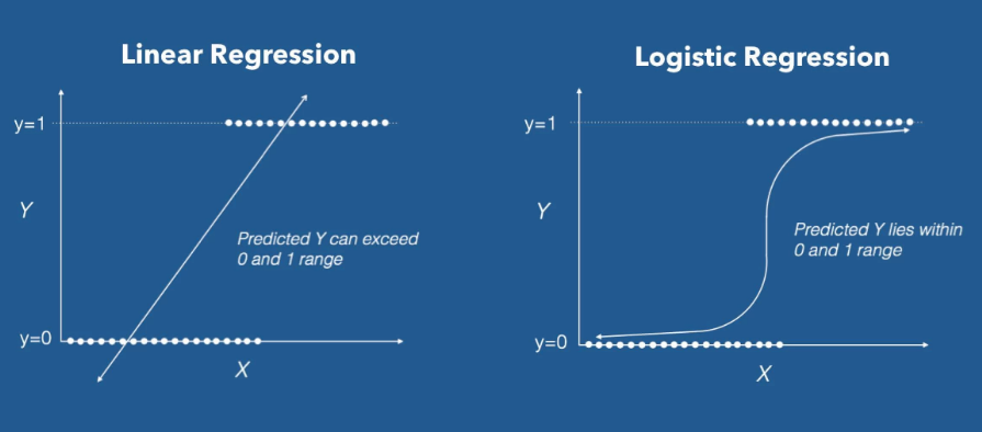
이진 분류 문제에서 로지스틱 회귀는 시그모이드 함수를 통과한 확률에 해당하는 출력값에 0.5와 같은 임계값(threshold)을 기준으로 분류합니다.
다중 분류 문제에서도 시그모이드 함수를 이용할 수 있을까요?
이진 분류의 경우 하나의 출력으로 두 클래스에 대한 확률을 모두 알 수 있습니다. ($A$ 일 확률 $p$, $B$ 일 확률 $1 - p$) 하지만 소프트맥스 회귀에서는 입력된 데이터에 대해 하나의 출력으로 바로 특정 클래스를 예측하는 것이 아니라 각 클래스에 대한 확률을 출력하여 가장 높은 확률을 갖는 클래스로 예측하는 것입니다. 따라서 출력의 합이 1이 되어야 하기 때문에 시그모이드 함수를 사용할 수 없는 것입니다.
소프트맥스 함수(Softmax Function)
소프트맥스 함수는 활성화 함수(activation function)의 한 종류로 출력의 합을 1로 만드는데 이것을 출력 강도를 정규화한다고 합니다.
3개의 출력에 대한 식으로 나타내면 다음과 같습니다.($e$ 는 자연 상수, $z$ 는 입력)
$z_1 \rightarrow {e^{z_1} \over e^{z_1}+e^{z_2}+e^{z_3}}$
$z_2 \rightarrow {e^{z_1} \over e^{z_1}+e^{z_2}+e^{z_3}}$
$z_3 \rightarrow {e^{z_1} \over e^{z_1}+e^{z_2}+e^{z_3}}$
$z_1+z_2+z_3=1$
import numpy as np

def softmax(array):
    r = []
    for z in sigmoid(array):
        r.append(np.exp(z) / sum(np.exp(sigmoid(array))))
    return r

a = np.array([0.3, 2.6, 4.1])

print(softmax(a))
print(sum(softmax(a)))
[0.25420056710998096, 0.36305075758862626, 0.38274867530139284]
1.0
원-핫 인코딩(One-Hot Encoding)
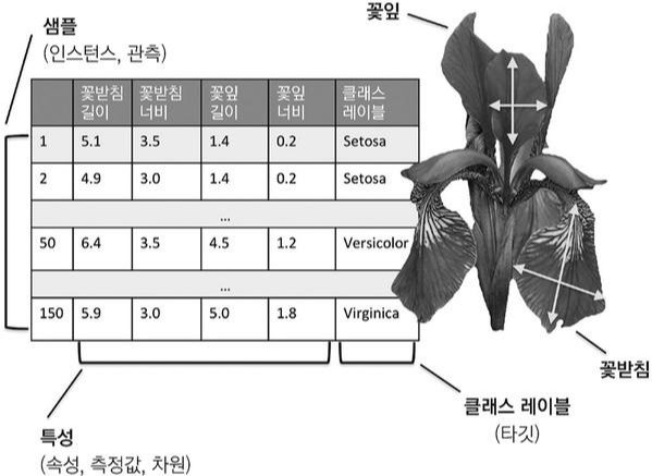
사용할 데이터는 붓꽃 데이터셋으로 타겟의 구성값을 확인합니다.
import numpy as np
from sklearn.datasets import load_iris

iris = load_iris()
data = iris.data
target = iris.target

np.unique(target, return_counts=1)
(array([0, 1, 2]), array([50, 50, 50], dtype=int64))
3개의 클래스를 가지며 값은 0,1,2 로 정수 인코딩되어있습니다. 신경망에 입력될 때는 정수 인코딩된 값을 원-핫 인코딩하여 각 클래스간의 관계를 균등하게 합니다.
넘파이에서는 단위 행렬을 생성하는 np.eye 를 이용할 수 있습니다.
np.eye(3, 7)array([[1., 0., 0., 0., 0., 0., 0.],
[0., 1., 0., 0., 0., 0., 0.],
[0., 0., 1., 0., 0., 0., 0.]])
다음과 같이 사용하면 입력 데이터에 대해 원-핫 인코딩할 수 있습니다.
label_size = np.unique(target).size

np.eye(label_size)[target]
array([[1., 0., 0.],
[1., 0., 0.],
[1., 0., 0.],
...
[0., 1., 0.],
[0., 1., 0.],
[0., 1., 0.],
...
[0., 0., 1.],
[0., 0., 1.],
[0., 0., 1.]])
텐서플로에서 제공하는 tf.keras.utils.to_categorical 을 이용하면 더욱 간단합니다.
import tensorflow as tf

tf.keras.utils.to_categorical(target)
array([[1., 0., 0.],
[1., 0., 0.],
[1., 0., 0.],
...
[0., 1., 0.],
[0., 1., 0.],
[0., 1., 0.],
...
[0., 0., 1.],
[0., 0., 1.],
[0., 0., 1.]])
또한 신경망 내부적으로 처리할 때는 텐서를 반환하는 tf.one_hot 을 이용할 수 있습니다.
import numpy as np
import tensorflow as tf

label_size = 5

x = tf.placeholder(tf.int32)
onehot = tf.one_hot(x, label_size)

with tf.Session() as sess:
    sess.run(tf.global_variables_initializer())

    print(sess.run(onehot, {x: [1, 4, 0, 2, 3]}))
[[0. 1. 0. 0. 0.]
[0. 0. 0. 0. 1.]
[1. 0. 0. 0. 0.]
[0. 0. 1. 0. 0.]
[0. 0. 0. 1. 0.]]
손실 함수(Loss Function)
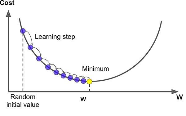
다중 클래스 분류 문제에서는 손실 함수로 크로스 엔트로피(cross-entropy)가 사용됩니다. 크로스 엔트로피는 정답 분포 $q$ 와 예측 분포 $p$ 사이의 평균 정보량을 의미합니다. 정보량은 해당 사건이 일어날 확률이 낮으면 증가하고 높으면 감소하게 되는데, 경사 하강법 최적화 알고리즘을 통해 그 정보량을 감소시켜 확률을 높이게 되는 것입니다.
크로스 엔트로피 손실 함수와 로지스틱 회귀에서의 손실 함수는 매우 유사합니다.
$L=-{1 \over n}\displaystyle \sum_{i=1}^n[y_i \text{log}(p_i)+(1-y_i) \text{log}(1-p_i)]$
이는 2개의 클래스를 갖는 이진 분류 문제에 대한 식으로 정답값이 0인 경우와 1인 경우를 고려한 것입니다. 다중 클래스 분류 문제에 대한 식도 이와 비슷합니다. 신경망에 입력되는 타겟 벡터는 원-핫 인코딩된 것으로 정답 클래스의 값은 1이고 나머지는 0입니다.
다음과 같이 클래스의 개수만큼 더해주어 나타낼 수 있습니다. ($k$는 클래스의 개수, $p$는 해당 클래스의 확률값, $y$는 원-핫 인코딩된 타겟 벡터)
$L=-\displaystyle \sum_{j=1}^ky_j \text{log}(p_j)$
최종적으로 n개의 데이터에 대한 식으로 나타내면 다음과 같습니다.
$L=-{1 \over n}\displaystyle \sum_{i=1}^n \sum_{j=1}^k y_{ij} \text{log}(p_{ij})$
텐서플로에서 제공하는 tf.nn.softmax_cross_entropy_logits_v2 를 이용하면 간단합니다.
import tensorflow as tf

x = tf.placeholder(tf.float32, [None, 1])
y = tf.placeholder(tf.float32, [None, 3])

output = tf.layers.dense(x, 3)

cross_entropy = -tf.reduce_sum(y * tf.log(tf.nn.softmax(output)), 1)
cross_entropy2 = tf.nn.softmax_cross_entropy_with_logits_v2(logits=output, labels=y)

with tf.Session() as sess:
    sess.run(tf.global_variables_initializer())

    _cross_entropy, _cross_entropy2 = sess.run([cross_entropy, cross_entropy2], {x: [[0.1], [0.2]], y: [[1., 0., 0.], [0., 1., 0.]]})

    print(_cross_entropy)
    print(_cross_entropy2)
[1.0372838 1.0633986]
[1.0372838 1.0633986]
구현
소프트맥스 회귀 모델을 구현합니다.
붓꽃 데이터셋을 불러옵니다.
from sklearn.datasets import load_iris

iris = load_iris()
data = iris.data
target = iris.target
feature_names = iris.feature_names
target_names = iris.target_names

print('data shape:', data.shape)
print('data sample:', data[0])
print('feature names:', feature_names)

print('target shape:', target.shape)
print('target sample:', target[0], target[1], target[2])
print('target label:', np.unique(target, return_counts=True))
print('target names:', target_names)
data shape: (150, 4)
data sample: [5.1 3.5 1.4 0.2]
feature names: ['sepal length (cm)', 'sepal width (cm)', 'petal length (cm)', 'petal width (cm)']
target shape: (150,)
target sample: 0 0 0
target label: (array([0, 1, 2]), array([50, 50, 50], dtype=int64))
target names: ['setosa' 'versicolor' 'virginica']
레이블은 3개의 클래스를 가지며 고르게 분포되어 있습니다.
target label: (array([0, 1, 2]), array([50, 50, 50], dtype=int64))
8:2 비율로 학습 데이터와 테스트 데이터로 분할합니다.
from sklearn.model_selection import train_test_split

x_train, x_test, y_train, y_test = train_test_split(data, target, test_size=0.2)
신경망을 정의합니다.
import numpy as np
import tensorflow as tf

class Model:
    def __init__(self, lr=1e-2):
        tf.reset_default_graph()

        with tf.name_scope('input'):
            self.x = tf.placeholder(tf.float32, [None, 4])
            self.y = tf.placeholder(tf.int64)

        with tf.name_scope('y_onehot'):
            y_onehot = tf.one_hot(self.y, 3)

        with tf.name_scope('layer'):
            fc = tf.layers.dense(self.x, 32, tf.nn.relu)
            logits = tf.layers.dense(fc, 3)

        with tf.name_scope('output'):
            h = tf.nn.softmax(logits)
            self.predict = tf.argmax(h, 1)

        with tf.name_scope('accuracy'):
            self.accuracy = tf.reduce_mean(tf.cast(tf.equal(tf.to_int64(self.predict), self.y), dtype=tf.float32))

        with tf.name_scope('loss'):
            cross_entropy = tf.nn.softmax_cross_entropy_with_logits_v2(logits=logits, labels=y_onehot)
            self.loss = tf.reduce_mean(cross_entropy)

        with tf.name_scope('optimizer'):
            self.train_op = tf.train.GradientDescentOptimizer(lr).minimize(self.loss)

        with tf.name_scope('summary'):
            tf.summary.scalar('loss', self.loss)
            tf.summary.scalar('accuracy', self.accuracy)

            self.merge = tf.summary.merge_all()

        self.writer = tf.summary.FileWriter('./tmp/softmax-regression_iris', tf.get_default_graph())

        self.sess = tf.Session()

        self.sess.run(tf.global_variables_initializer())

    def train(self, x_train, y_train, epochs):
        for e in range(epochs):
            summary, loss, accuracy, _ = self.sess.run([self.merge, self.loss, self.accuracy, self.train_op], {self.x: x_train, self.y: y_train})
            self.writer.add_summary(summary, e)
            print('epoch:', e + 1, ' / loss:', loss, '/ accuracy:', accuracy)

    def score(self, x, y):
        return self.sess.run(self.accuracy, {self.x: x, self.y: y})
배치 경사 하강법으로 학습을 수행합니다.
def train(self, x_train, y_train, epochs):
    for e in range(epochs):
        summary, loss, accuracy, _ = self.sess.run([self.merge, self.loss, self.accuracy, self.train_op], {self.x: x_train, self.y: y_train})
        self.writer.add_summary(summary, e)
        print('epoch:', e + 1, ' / loss:', loss, '/ accuracy:', accuracy)
모델을 학습하고 테스트합니다.
model = Model()
model.train(x_train, y_train, epochs=500)
model.score(x_test, y_test)
...
epoch: 490 / loss: 0.25155848 / accuracy: 0.9583333
epoch: 491 / loss: 0.25125748 / accuracy: 0.9583333
epoch: 492 / loss: 0.2509577 / accuracy: 0.9583333
epoch: 493 / loss: 0.2506586 / accuracy: 0.9583333
epoch: 494 / loss: 0.25035974 / accuracy: 0.9583333
epoch: 495 / loss: 0.25006163 / accuracy: 0.9583333
epoch: 496 / loss: 0.24976416 / accuracy: 0.9583333
epoch: 497 / loss: 0.24946807 / accuracy: 0.9583333
epoch: 498 / loss: 0.24917193 / accuracy: 0.9583333
epoch: 499 / loss: 0.24887681 / accuracy: 0.9583333
epoch: 500 / loss: 0.24858236 / accuracy: 0.9583333
0.96666664
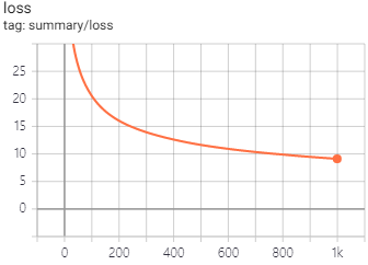
에포크에 대한 정확도와 손실 함수의 그래프는 다음과 같습니다.

'머신러닝 > 딥러닝' 카테고리의 다른 글
| 순환 신경망(Recurrent Neural Network) (1) (0) | 2020.11.16 |
|---|---|
| 합성곱 신경망(Convolutional Neural Network) (0) | 2020.11.13 |
| 교차 검증(Cross Validation) (0) | 2020.11.09 |
| 로지스틱 회귀(Logistic Regression) (0) | 2020.11.06 |
| 선형 회귀(Linear Regression) (0) | 2020.11.06 |