A3C(Asynchronous Advantage Actor-Critic)
논문 Asynchronous Methods for Deep Reinforcement Learning 으로 소개되었습니다.
A2C 는 온라인 학습과 어드밴티지를 통해 분산을 줄였지만 여전히 문제를 가지고 있습니다. (A2C 단일 에이전트) 학습에 사용하는 샘플 데이터들은 시간의 흐름에 따라 순차적인 것으로 데이터들이 서로 연관된 것입니다. 이러한 데이터간의 높은 상관관계(correlation)는 목적 함수의 그래디언트를 편향시키고 학습을 불안정하게 만들 수 있습니다.
A3C 는 비동기(asynchronous)라는 의미가 추가된 것으로 다중 에이전트를 통해 비동기적으로 공유 신경망을 학습하는 방법론입니다. 각 에이전트는 독립적인 환경에서 에피소드를 수행하며 얻은 샘플 데이터를 이용하여 공유 신경망의 파라미터를 업데이트하고 그 파라미터를 자신의 네트워크로 복제하는 과정을 통해 학습하는 것입니다.
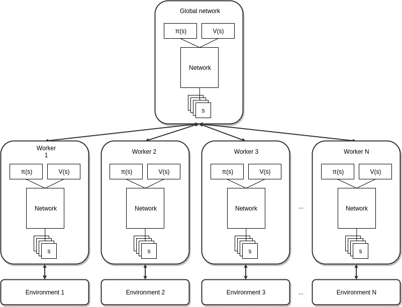
이러한 다중 에이전트를 병렬적으로 운용함에 따라 수집되는 데이터의 다양성은 증가하게 되어 데이터간의 상관관계를 줄일 수 있다는 것입니다.
또한 목적 함수 그래디언트 계산에 엔트로피(entropy)를 추가하는데 이는 조기 수렴을 막아 탐색(exploration)이 향상된다는 것입니다.
엔트로피(Entropy)
먼저 정보량은 다음과 같이 정의됩니다.
$h(x) = - \text{log} \, p(x)$
이는 빈번하게 일어나는 사건은 새로울 것이 없으므로 정보량은 적으며 반대로 빈번하지 않은 사건은 정보량이 많다는 것입니다.
엔트로피는 정보량의 기댓값으로 정의됩니다.
$H(p) = E_{x \thicksim p(x)}[ - \text{log} \, p(x) ] = -\int_x p(x) \, \text{log} \, p(x) dx$
$p(x)$ 가 다음과 같이 평균이 $\mu$ 이고 표준 편차가 $\sigma$ 인 확률 밀도 함수라면
$p(x) \doteq {1 \over \sigma \sqrt{2 \pi}} \text{exp} \left( - { (x \, - \, \mu)^2 \over 2 \sigma^2 } \right)$
엔트로피는 다음과 같습니다.
$H(p) = {1 \over 2} (1 + \text{log} (2\pi \sigma^2))$
이 경우 엔트로피는 분산 $\sigma^2$ 에만 영향을 받으며 분산이 커질수록 증가하는 것입니다. 분산이 커질수록 사건의 무작위성이 커지고 특정 사건의 발생 빈도수가 작아지기 때문에 정보량이 증가하는 것입니다.
이에 따라 엔트로피를 추가한 목적 함수의 그래디언트 식은 다음과 같습니다.
$\nabla_{\theta'} J(\theta') = \nabla_{\theta'} \text{log} \pi(a_t|s_t; \theta')(R_t - V(s_t; \theta'_v)) + \beta \nabla_{\theta'} H(\pi(s_t; \theta'))$
추가된 엔트로피에 의해 확률 분포는 영향을 받게 되는데 하이퍼 파라미터 $\beta$ 로 탐색(exploration)과 활용(exploitation) 사이를 제어할 수 있습니다. $\beta$ 를 큰 값으로 하면 그래디언트 계산에 엔트로피의 영향력이 커져 무작위성이 증가하게 되고 $\beta$ 를 작은 값으로 하면 그에 대한 영향력은 작아지게 되는 것입니다.
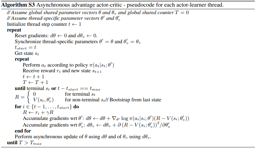
알고리즘
구현
알고리즘 테스트 환경은 OpenAI Gym 의 Pendulum-v0 입니다.

Pendulum 는 연속적인 행동 공간을 갖는 문제로 진자를 흔들어서 12시 방향으로 세워서 유지하는 문제입니다.
환경으로부터 받을 수 있는 정보를 출력합니다.
import gym

env = gym.make('Pendulum-v0')

print('obs:', env.observation_space.shape[0])
print('act:', env.action_space.shape[0])
print('act bound:', env.action_space.low[0], env.action_space.high[0])
상태 정보는 3차원의 벡터로 연속적인 공간을 갖으며 에이전트가 취할 수 있는 행동 또한 [-2, 2] 의 범위의 연속적인 공간을 갖습니다.
obs: 3
act: 1
act bound: -2.0 2.0
신경망을 정의합니다.
def build_net(self, scope):
    with tf.variable_scope('actor'):
        a_fc1 = tf.layers.dense(self.s, 512, tf.nn.relu)
        a_fc2 = tf.layers.dense(a_fc1, 256, tf.nn.relu)
        mu = tf.layers.dense(a_fc2, N_A, tf.nn.tanh) * A_BOUND[1]
        sigma = tf.layers.dense(a_fc2, N_A, tf.nn.softplus)

    with tf.variable_scope('critic'):
        c_fc1 = tf.layers.dense(self.s, 512, tf.nn.relu)
        c_fc2 = tf.layers.dense(c_fc1, 256, tf.nn.relu)
        v = tf.layers.dense(c_fc2, 1)

    a_params = tf.get_collection(tf.GraphKeys.TRAINABLE_VARIABLES, scope + '/actor')
    c_params = tf.get_collection(tf.GraphKeys.TRAINABLE_VARIABLES, scope + '/critic')

    return a_params, c_params, v, mu, sigma
액터 신경망의 출력층으로 확률 밀도 함수를 나타내는 평균과 표준 편차를 출력합니다.
mu = tf.layers.dense(a_fc2, N_A, tf.nn.tanh) * A_BOUND[1]
sigma = tf.layers.dense(a_fc2, N_A, tf.nn.softplus)
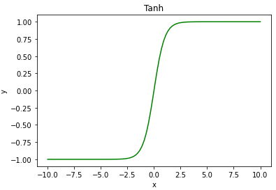
활성화 함수 tanh 은 [-1, 1] 의 범위를 갖기 때문에 환경이 갖는 행동 범위 [-2, 2] 로 조정합니다.
A_BOUND = [env.action_space.low, env.action_space.high]

...

mu = tf.layers.dense(a_fc2, N_A, tf.nn.tanh) * A_BOUND[1]
tanh 함수는 sigmoid 를 변환해서 나온 함수입니다.
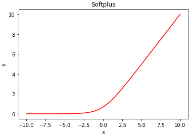
표준 편차에는 활성화 함수 softplus 를 이용합니다.
sigma = tf.layers.dense(a_fc2, N_A, tf.nn.softplus)
softplus 함수는 부드러운 ReLU 라고 할 수 있습니다.
스코프를 통해 공유 신경망과 일반 신경망을 구분합니다.
if scope == 'global':
    with tf.variable_scope(scope):
        with tf.name_scope('input'):
            self.s = tf.placeholder(tf.float32, [None, N_S], name='state')
        self.a_params, self.c_params = self.build_net(scope)[:2]
else:
    with tf.variable_scope(scope):
        with tf.name_scope('input'):
            self.s = tf.placeholder(tf.float32, [None, N_S], name='state')
            self.a = tf.placeholder(tf.float32, [None, N_A], name='action')
            self.td_target = tf.placeholder(tf.float32, [None, 1], name='td_target')

        self.a_params, self.c_params, self.v, self.mu, self.sigma = self.build_net(scope)
크리틱 신경망의 손실 함수를 정의합니다.
with tf.name_scope('td_error'):
    self.td_error = self.td_target - self.v
with tf.name_scope('c_loss'):
    self.c_loss = tf.reduce_mean(tf.square(self.td_error))
TD 오차를 계산한 후 제곱의 평균을 계산하는 것으로 계산된 TD 오차는 어드밴티지로 사용합니다.
실수 범위를 갖는 행동을 선택합니다.
with tf.name_scope('output'):
    self.dist = tf.distributions.Normal(self.mu, self.sigma)
    self.sample = self.dist.sample()
    self.action = tf.clip_by_value(self.sample, *A_BOUND)
출력층의 평균과 표준 편차로 가우시안 분포를 구합니다. (tf.distributions.Normal)
self.dist = tf.distributions.Normal(self.mu, self.sigma)
가우시안 분포로 부터 샘플을 선택하고 범위를 클리핑하여 행동을 구합니다.
self.sample = self.dist.sample()
self.action = tf.clip_by_value(self.sample, *A_BOUND)
액터 신경망의 손실 함수를 정의합니다.
with tf.name_scope('a_loss'):
    self.a_loss = self.dist.log_prob(self.a) * tf.stop_gradient(self.td_error) + self.dist.entropy() * ENTROPY_BETA
tf.stop_gradient 를 사용한 것은 공통된 입력층을 통해 입력받아 액터와 크리틱 신경망을 동시에 업데이트하기 때문에 TD 오차 계산과 관련된 크리틱의 파라미터에 대한 그래디언트 계산을 중지하는 것입니다.
공유 신경망과 일반 신경망간의 업데이트를 정의합니다.
with tf.name_scope('local_grad'):
    self.a_grads = tf.gradients(self.a_loss, self.a_params)
    self.c_grads = tf.gradients(self.c_loss, self.c_params)

with tf.name_scope('pull'):
    self.a_pull_op = [l_p.assign(g_p) for l_p, g_p in zip(self.a_params, globalAC.a_params)]
    self.c_pull_op = [l_p.assign(g_p) for l_p, g_p in zip(self.c_params, globalAC.c_params)]
with tf.name_scope('push'):
    self.a_push_op = tf.train.RMSPropOptimizer(LR_A).apply_gradients(zip(self.a_grads, globalAC.a_params))
    self.c_push_op = tf.train.RMSPropOptimizer(LR_C).apply_gradients(zip(self.c_grads, globalAC.c_params))

...

def update_global(self, feed_dict):
    self.sess.run([self.c_push_op, self.a_push_op], feed_dict)

def pull_global(self):
    self.sess.run([self.c_pull_op, self.a_pull_op])
일반 신경망의 그래디언트 계산을 정의합니다.(tf.gradients)
with tf.name_scope('local_grad'):
    self.a_grads = tf.gradients(-self.a_loss, self.a_params)
    self.c_grads = tf.gradients(self.c_loss, self.c_params)
글로벌 신경망의 파라미터를 일반 신경망의 파라미터로 복제하는 부분입니다.
with tf.name_scope('pull'):
    self.a_pull_op = [l_p.assign(g_p) for l_p, g_p in zip(self.a_params, globalAC.a_params)]
    self.c_pull_op = [l_p.assign(g_p) for l_p, g_p in zip(self.c_params, globalAC.c_params)]
그래디언트와 적용할 파라미터를 설정합니다.(tf.train.Optimizer)
with tf.name_scope('push'):
    self.a_push_op = tf.train.RMSPropOptimizer(LR_A).apply_gradients(zip(self.a_grads, globalAC.a_params))
    self.c_push_op = tf.train.RMSPropOptimizer(LR_C).apply_gradients(zip(self.c_grads, globalAC.c_params))
일반 신경망의 파라미터를 통해 그래디언트를 계산하고 글로벌 신경망의 파라미터를 업데이트하는 것입니다.
$\theta = \theta + \nabla_{\theta'} J(\theta')$
쓰레드를 통해 독립적으로 에피소드를 진행하는 각 에이전트는 공유 파라미터를 이용해 업데이트를 수행하고 다시 일반 신경망의 파라미터로 복제함으로써 공유하는 것입니다.
쓰레드를 통해 다중 에이전트에 학습을 수행합니다.(tf.train.Coordinator)
sess = tf.Session(config=config)
coord = tf.train.Coordinator()

workers = []
with tf.device('/cpu:0'):
    globalAC = A3C('global')
    for i in range(16):
        name = 'worker_%i' % i
        workers.append(A3C(name, globalAC, sess, coord, max_epi))

sess.run(tf.global_variables_initializer())

worker_threads = []
for w in workers:
    t = threading.Thread(target=w.run)
    t.start()
    worker_threads.append(t)

coord.join(worker_threads)
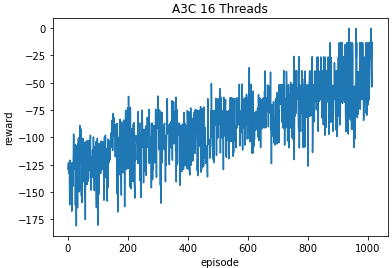
1000번의 에피소드 동안 학습한 결과입니다.
'머신러닝 > 강화학습' 카테고리의 다른 글
| PPO(Proximal Policy Optimization) (0) | 2020.12.07 |
|---|---|
| DDPG(Deep Deterministic Policy Gradient) (0) | 2020.11.30 |
| 액터-크리틱(Actor-Critic) (0) | 2020.11.27 |
| 정책 그래디언트(Policy Gradient) (0) | 2020.11.24 |
| DQN(Deep Q-Networks) (2) (0) | 2020.11.24 |