선형 회귀(Linear Regression)

종속 변수 $y$ 와 하나 이상의 독립 변수 $x$ 와의 선형 관계를 모델링하는 통계학 기법입니다. 변수 $x$ 의 값은 독립적으로 변할 수 있으나 $y$ 의 값은 $x$ 의 값에 의해 종속적으로 결정됩니다.

 

1개의 독립 변수를 갖는 단순 선형 회귀(simple linear regression)의 수식은 다음과 같습니다.

 

$y=Wx+b$

 

이는 직선 방정식으로 $W$ 는 기울기, $b$ 는 절편이며 신경망의 파라미터(parameter)로 각각 가중치(weight)와 편향(bias)을 의미합니다.

 

 

즉 입력 데이터에 대한 예측으로 직선을 구하는 문제라고 할 수 있습니다.

 

 

2개 이상의 독립 변수를 다루면 이를 다중 선형 회귀(multiple linear regression)라고 합니다.

 

$y=W_0x_0+W_1x_1+...W_nx_n+b$

 

이는 데이터가 갖는 다수의 특성(feature) $x_0, ..., x_n$ 을 고려하여 $y$ 를 예측하는 것입니다. 입력 데이터는 n차원을 갖는 벡터로 데이터의 특성의 개수와 가중치의 개수는 같아야 합니다.

 

 

행렬의 곱

다음과 같은 다중 선형 회귀의 수식은 벡터의 내적 또는 행렬의 곱으로 나타낼 수 있습니다.

 

$y=W_0x_0+W_1x_1+...W_nx_n+b$

 

이는 데이터의 개수와 관련이 있는데 1개의 입력 데이터 $ [ x_0\ x_1\ x_2\ \cdots\ x_n  ] $ 에 대한 연산은 벡터의 내적으로 표현할 수 있습니다.

 

$
y =   
\left[  
    \begin{array}{c}  
      x_{0}\ x_{1}\ x_{2}\ \cdots\ x_{n}  
    \end{array}  
  \right]  
\left[  
    \begin{array}{c}  
      W_{0} \\  
      W_{1} \\  
      W_{2} \\  
      \cdot\cdot\cdot \\  
      W_{n}  
    \end{array}  
  \right]  
+  
b
= x_0W_0 + x_1W_1 + x_2W_2 + ... + x_nW_n + b 
$

입력 데이터가 여러 개인 경우 행렬의 곱으로 표현할 수 있습니다.

$\left[   
    \begin{array}{c}   
      x_{11}\ x_{12}\ x_{13}\ x_{14} \\   
      x_{21}\ x_{22}\ x_{23}\ x_{24} \\   
      x_{31}\ x_{32}\ x_{33}\ x_{34} \\   
      x_{41}\ x_{42}\ x_{43}\ x_{44} \\   
      x_{51}\ x_{52}\ x_{53}\ x_{54} \\   
    \end{array}   
  \right]   
\left[   
    \begin{array}{c}   
      w_{1} \\   
      w_{2} \\   
      w_{3} \\   
      w_{4} \\   
    \end{array}   
  \right]  

  +  

\left[   
    \begin{array}{c}   
      b \\   
      b \\   
      b \\   
      b \\

      b \\   
    \end{array}   
  \right]  
  =   
\left[   
    \begin{array}{c}   
      x_{11}w_{1}+ x_{12}w_{2}+ x_{13}w_{3}+ x_{14}w_{4} + b \\   
      x_{21}w_{1}+ x_{22}w_{2}+ x_{23}w_{3}+ x_{24}w_{4} + b \\   
      x_{31}w_{1}+ x_{32}w_{2}+ x_{33}w_{3}+ x_{34}w_{4} + b \\   
      x_{41}w_{1}+ x_{42}w_{2}+ x_{43}w_{3}+ x_{44}w_{4} + b \\   
      x_{51}w_{1}+ x_{52}w_{2}+ x_{53}w_{3}+ x_{54}w_{4} + b \\   
    \end{array}   
  \right]$

 

넘파이의 np.dot 을 이용하면 두 행렬간의 곱 연산을 수행할 수 있습니다.

import numpy as np

a = np.arange(20).reshape(5, 4)
b = np.array([1, -1, 1, -1, 0, 0, 0, 0]).reshape(-1, 2)

r = np.dot(a, b)

print(a)
print(b)
print(r)

[[ 0  1  2  3]
 [ 4  5  6  7]
 [ 8  9 10 11]
 [12 13 14 15]
 [16 17 18 19]]
[[ 1 -1]
 [ 1 -1]
 [ 0  0]
 [ 0  0]]
[[  1  -1]
 [  9  -9]
 [ 17 -17]
 [ 25 -25]
 [ 33 -33]]

 

 

데이터 전처리

신경망에 입력되는 데이터가 여러 특성을 갖을 경우에는 각 특성의 데이터 분포를 확인해야 합니다. 주어지는 데이터는 항상 신경망 학습을 위해 특화되어 있지 않으며 특성에 따라 구성된 값의 단위가 다르다는 것입니다.

 

데이터의 스케일을 조정하는 방법에는 표준화(standardization)와 정규화(normalization)가 있습니다.

 

표준화는 데이터를 평균 $ \mu $ 이 0이고 표준 편차 $ \sigma $ 가 1인 분포로 만들어주는 것입니다.

 

$ X = { X - \mu \over \sigma} $ 

 

정규화는 스케일의 범위를 $ [0, 1] $ 로 만들어 주는 것입니다. 

 

$ X = { X - X_{min} \over X_{max} - X_{min} } $

 

특성의 영향을 균등하게 하는 것이라고 할 수 있습니다.

 

테스트 데이터를 산점도를 통해 비교해보면 기존 분포의 모양을 유지하며 y축의 스케일이 조정된 것을 확인할 수 있습니다.(실제 데이터는 y축이 아닌 x축 데이터를 전처리합니다.)

import numpy as np
import matplotlib.pyplot as plt

x = 500
y = np.random.normal(0, 10, x)

fig = plt.figure(figsize=(16, 4))

plt.subplot(131)
plt.scatter(range(x), y)
plt.title('Raw')

plt.subplot(132)
y_std = (y - y.mean()) / y.std()
plt.scatter(range(x), y_std, color='red')
plt.title('Standardization')

plt.subplot(133)
y_norm = (y - y.min()) / (y.max() - y.min())
plt.scatter(range(x), y_norm, color='green')
plt.title('Normalization')

plt.show()

 

 

손실 함수(Loss Function)

회귀 문제에서 손실 함수는 주로 평균 제곱 오차(mean squared error, MSE)가 사용되며 정답 $y$ 과 예측 $\hat y$ 의 오차 또는 손실을 최소화(minimize)하는 방향으로 파라미터를 학습합니다.

 

$MSE={1 \over n}\displaystyle \sum_{i=1}^n (y_i-\hat y_i)^2$

 

 

구현

다중 선형 회귀 모델을 구현합니다.

 

보스턴 주택 가격 데이터셋을 불러옵니다.

from sklearn.datasets import load_boston

boston = load_boston()

data = boston.data
target = boston.target
feature_names = boston.feature_names

print('data shape:', data.shape)
print('data sample:', data[0])
print('feature_names:', feature_names)

print('target shape:', target.shape)
print('target sample:', target[0], target[1], target[2])

data shape: (506, 13)
data sample: [6.320e-03 1.800e+01 2.310e+00 0.000e+00 5.380e-01 6.575e+00 6.520e+01
 4.090e+00 1.000e+00 2.960e+02 1.530e+01 3.969e+02 4.980e+00]
feature_names: ['CRIM' 'ZN' 'INDUS' 'CHAS' 'NOX' 'RM' 'AGE' 'DIS' 'RAD' 'TAX' 'PTRATIO'
 'B' 'LSTAT']
target shape: (506,)
target sample: 24.0 21.6 34.7

 

신경망에 정의한 입력 타겟의 형태는 다음과 같습니다.

self.y = tf.placeholder(tf.float32, [None, 1])

 

따라서 기존 타겟 데이터의 형태 변형이 필요합니다.

target = target.reshape(-1, 1)
target.shape

(506, 1)

 

8:2의 비율로 학습 데이터와 테스트 데이터로 분할합니다.

from sklearn.model_selection import train_test_split

x_train, x_test, y_train, y_test = train_test_split(data, target, test_size=0.2)

 

데이터 분포를 확인합니다.

import matplotlib.pyplot as plt

fig = plt.figure(figsize=(12, 6))
ax = fig.add_subplot(111)

for i in range(x_train.shape[1]): # all features
    ax.scatter(x_train[:, i], y_train, s=10)
    
plt.title('Raw')
plt.xlabel('x')
plt.ylabel('y')
plt.show()

 

산점도 상에 나타난 각 특성의 스케일은 0에서 700정도로 넓게 분포합니다. 안정적인 학습을 위해서는 전처리가 필요합니다.

 

표준화를 위해 학습 데이터의 평균과 표준 편차를 구합니다.

train_mean = x_train.mean(axis=0)
train_std = x_train.std(axis=0)

 

평균과 표준 편차를 이용해 학습 데이터와 테스트 데이터를 표준화합니다. 

x_train = (x_train - train_mean) / train_std
x_test = (x_test - train_mean) / train_std

 

주의할 점은 테스트 데이터를 전처리할 때도 학습 데이터의 통계를 이용한다는 것입니다. 테스트 데이터는 최종 성능 평가를 위한 것으로 어떠한 정보도 누출되어서는 안됩니다.

 

산점도로 나타나는 x축의 스케일이 조정되었습니다.

import matplotlib.pyplot as plt

fig = plt.figure(figsize=(12, 6))
ax = fig.add_subplot(111)

for i in range(x_train.shape[1]): # all features
    ax.scatter(x_train[:, i], y_train, s=10)
    
plt.title('Standardization')
plt.xlabel('x')
plt.ylabel('y')
plt.show()

 

신경망을 정의합니다.

import numpy as np
import tensorflow as tf

class Model:
    def __init__(self, lr=1e-3):
        with tf.name_scope('input'):
            self.x = tf.placeholder(tf.float32, [None, 13])
            self.y = tf.placeholder(tf.float32, [None, 1])

        with tf.name_scope('layer'):
            w = tf.Variable(tf.random_normal([13, 64]))
            b = tf.Variable(tf.random_normal([1]))

            z = tf.matmul(self.x, w) + b
            h = tf.nn.relu(z)

            w2 = tf.Variable(tf.random_normal([64, 1]))
            b2 = tf.Variable(tf.random_normal([1]))

        with tf.name_scope('output'):
            pred = tf.matmul(h, w2) + b2

        with tf.name_scope('loss'):
            self.loss = tf.losses.mean_squared_error(self.y, pred)

        with tf.name_scope('optimizer'):
            self.train_op = tf.train.GradientDescentOptimizer(lr).minimize(self.loss)

        with tf.name_scope('summary'):
            tf.summary.scalar('loss', self.loss)
            self.merge = tf.summary.merge_all()

        self.writer = tf.summary.FileWriter('./tmp/linear-regression', tf.get_default_graph())
        
        self.sess = tf.Session()
        
        self.sess.run(tf.global_variables_initializer())
                               
    def train(self, x, y, epochs):
        for e in range(epochs):
            summary, loss, _ = self.sess.run([self.merge, self.loss, self.train_op], {self.x: x, self.y: y})
            self.writer.add_summary(summary, e)
            print('epoch:', e + 1, ' / loss:', loss)
    
    def test(self, x, y):
        loss = self.sess.run(self.loss, {self.x: x, self.y: y})
        return loss

 

배치 경사 하강법으로 학습을 수행합니다.

def train(self, x, y, epochs):
    for e in range(epochs):
        summary, loss, _ = self.sess.run([self.merge, self.loss, self.train_op], {self.x: x, self.y: y})
        self.writer.add_summary(summary, e)
        print('epoch:', e + 1, ' / loss:', loss)

 

모델을 학습하고 테스트합니다.

model = Model()
model.train(x_train, y_train, epochs=1000)
model.test(x_test, y_test)

...

epoch: 990  / loss: 9.514389
epoch: 991  / loss: 9.510468
epoch: 992  / loss: 9.506571
epoch: 993  / loss: 9.502658
epoch: 994  / loss: 9.49877
epoch: 995  / loss: 9.494896
epoch: 996  / loss: 9.490974
epoch: 997  / loss: 9.4871645
epoch: 998  / loss: 9.483273
epoch: 999  / loss: 9.479406
epoch: 1000  / loss: 9.475529

14.222591

 

에포크에 대한 손실 함수의 그래프는 다음과 같습니다.

 

 

 

신경망(Neural Network)

신경망의 내부 동작은 추론 과정에 해당하는 순전파(forward-propagation)와 학습 과정에 해당하는 역전파(back-propagation)로 나누어집니다.

 

특히 역전파는 다층 퍼셉트론과 같은 은닉층(hidden layer)을 포함하는 신경망에서 경사 하강법(gradient descent)을 이용한 학습 과정으로 미분의 체인 룰(chain rule)을 통해 기울기가 역으로 전파되어 파라미터가 업데이트되는 원리입니다.

 

예제를 통해 순전파와 역전파의 계산 과정을 알아보겠습니다.

 

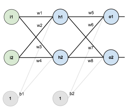
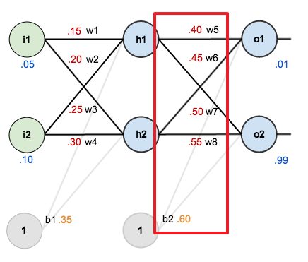
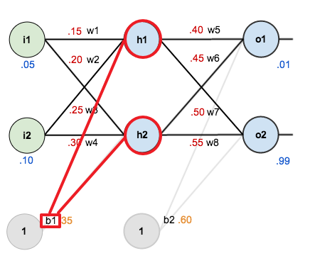
다음 신경망은 입력층, 은닉층, 출력층으로 구성되며 각 층은 2개의 노드를 가지고 있습니다.

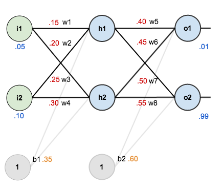
신경망에서 학습 가능한 파라미터는 가중치 $w_1$~$w_8$ 와 편향 $b_1, b_2$ 이며, 은닉층 노드 $h_1, h_2$ 와 출력층 노드 $o_1, o_2$ 에는 시그모이드 활성화 함수가 사용됩니다. 또한 손실 함수는 평균 제곱 오차를 사용하며 경사 하강법의 학습률은 0.5로 지정합니다.

 

초기 파라미터 값은 다음과 같습니다.

 

 

순전파(Forward-Propagation)

먼저 노드 $h_1$ 의 입력 $net_{h_1}$ 에 대해 계산합니다.

 

$ net_{h_1} = w_1 * i_1 + w_2 * i_2 + b_1 = 0.15 * 0.05 + 0.2 * 0.1 + 0.35 = 0.3775 $

 

$ net_{h_1} $ 을 시그모이드 함수를 통한 출력 $ out_{h_1} $ 은 다음과 같습니다.

 

$ out_{h_1} = {1 \over {1 + e^{net_{h_1}}} } = {1 \over {1 + e^{ -0.3775 }} } = 0.593269992 $

 

$ h_2 $ 도 같은 방식으로 계산합니다.

 

$ net_{h_2} = w_3 * i_1 + w_4 * i_2 + b_1 = 0.25 * 0.05 + 0.3 * 0.1 + 0.35 = 0.3925 $

 

$ out_{h_2} = {1 \over {1 + e^{net_{h_2}}} } = {1 \over {1 + e^{ -0.3925 }} } = 0.596884378 $

 

$ h_1, h_2 $ 에 대해 정리하면 다음과 같습니다.

 

$ net_{h_1} = 0.3775 $
$ net_{h_2} = 0.3925 $

$ out_{h_1} = 0.593269992 $

$ out_{h_2} = 0.596884378 $

 

 

위와 같은 방식으로 노드 $ o_1, o_2 $ 를 계산합니다.

 

$\begin{aligned}  
net_{o_1} & = w_5 * out_{h_1} + w_6 * out_{h_2} + b_2 \\\\  
& = 0.4 * 0.593269992 + 0.45 * 0.596884378 + 0.6 \\\\ 
& = 1.1059059669
\end{aligned}$

 

$ out_{o_1} = {1 \over {1 + e^{net_{o_1}}} } = {1 \over {1 + e^{ -1.1059059669 }} } = 0.7513650695224682 $

 

$\begin{aligned}   
net_{o_2} & = w_7 * out_{h_1} + w_8 * out_{h_2} + b_2 \\\\   
& = 0.5 * 0.593269992 + 0.55 * 0.596884378 + 0.6 \\\\  
& = 1.2249214039
\end{aligned}$ 

$ out_{o_2} = {1 \over {1 + e^{net_{o_2}}} } = {1 \over {1 + e^{ -1.2249214039 }} } = 0.772928465286981 $a

 

$o_1, o_2$ 에 대해 정리하면 다음과 같습니다.

 

$net_{o_1} = 1.1059059669$ 
$net_{o_2} = 1.2249214039 $
$out_{o_1} = 0.7513650695224682$
$out_{o_2} = 0.772928465286981 $

 

 

신경망의 출력과 타겟의 평균 제곱 오차를 계산합니다. 계산에 편의를 위해 $ 1 \over 2 $ 를 곱하며 1개의 입력에 대한 것이므로 다음과 같이 나타낼 수 있습니다.

 

$E = { 1\over 2 } (y - \hat y)^2 $

 

 

출력 $out_{o_1}$ 에 대한 타겟값은 $0.01$ 이며, $out_{o_2}$ 에 대한 타겟값은 $0.99$ 입니다.

 

$ target_{o_1} = 0.01 $

$ target_{o_2} = 0.99 $

 

$ E_{o_1} = { 1 \over 2 } ( target_{o_1} - out_{o_1} )^2 = { 1 \over 2 } ( 0.01 - 0.7513650695224682 )^2 = 0.274811083 $ 

 

$ E_{o_2} = { 1 \over 2 } ( target_{o_2} - out_{o_2} )^2 = { 1 \over 2 } ( 0.99 - 0.772928465286981 )^2 = 0.023560026 $ 

 

오차의 합을 계산합니다.

 

$ E_\text{total} = E_{o_1} + E_{o_2} = 0.274811083 + 0.023560026 = 0.298371109 $

 

역전파(Back-Propagation)

신경망에서 학습 가능한 파라미터는 가중치 $w_1$~$w_8$ 와 편향 $b_1, b_2$ 입니다. 이에 대해 경사 하강법을 적용하기 위해서는 먼저 각 파라미터에 대해 기울기를 계산해야 합니다.

 

우선 출력층에 가까운 $w_5$~$w_8$, $b_2$ 에 대해 업데이트를 진행합니다.

$w_5$ 에 대한 오차의 기울기 $\partial E_\text{total} \over \partial w_5$ 는 체인 룰에 의해 다음과 같이 나타낼 수 있습니다.

 

${\partial E_{total} \over \partial w_5} = {\partial E_\text{total} \over \partial out_{o_1}} {\partial out_{o_1} \over \partial net_{o_1}} {\partial net_{o_1} \over \partial w_5 }$

 

다음 항을 계산합니다.

 

${\partial E_\text{total} \over \partial w_5} = \color{red}{\partial E_\text{total} \over \partial out_{o_1}} {\partial out_{o_1} \over \partial net_{o_1}} {\partial net_{o_1} \over \partial w_5 }$

 

$\begin{aligned} 
{\partial E_\text{total} \over \partial out_{o_1}} & = { \partial \over \partial out_{o_1} } \left[ {1 \over 2}(target_{o_1} - out_{o_1} )^2 + {1 \over 2} ( target_{o_2} - out_{o_2} )^2 \right] \\\\
& = 2 * {1 \over 2}(target_{o_1} - out_{o_1}) * -1 + 0 \\\\ 
& = -(target_{o_1} - out_{o_1}) \\\\ 
& = -(0.01 - 0.7513650695224682) \\\\ 
& = 0.741365069 
\end{aligned}$

 

다음 항을 계산합니다.

 

${\partial E_\text{total} \over \partial w_5} = {\partial E_\text{total} \over \partial out_{o_1}} \color{red}{\partial out_{o_1} \over \partial net_{o_1}} {\partial net_{o_1} \over \partial w_5 }$

 

$ out_{o_1} $ 는 시그모이드 함수를 통한 출력입니다.

 

$ out_{o_1} = {1 \over { 1 + e^{-net_{o_1}} }} $

 

시그모이드 함수의 미분은 다음과 같습니다.

 

$ {\partial \over \partial x} \sigma (x) = \sigma (x) (1 - \sigma(x)) $

 

따라서 다음과 같이 계산할 수 있습니다.

 

$\begin{aligned} 
\partial out_{o_1} \over \partial net_{o_1} & = out_{o_1} ( 1 - out_{o_1} ) \\\\ 
& = 0.7513650695224682 ( 1 - 0.7513650695224682 ) \\\\ 
& = 0.186815602 
\end{aligned}$

 

다음 항을 계산합니다.

 

${\partial E_\text{total} \over \partial w_5} = {\partial E_\text{total} \over \partial out_{o_1}} {\partial out_{o_1} \over \partial net_{o_1}} \color{red}{\partial net_{o_1} \over \partial w_5 }$

 

$\begin{aligned} 
\partial net_{o_1} \over \partial w_5 & = { \partial \over \partial w_5 } (w_5 * out_{h_1} + w_6 * out_{h_2} + b_2) \\\\
& = 1 * out_{h_1} \\\\ 
& = 1 * 0.593269992 \\\\ 
& = 0.593269992 
\end{aligned}$

 

최종적으로 $ {\partial E_\text{total} \over \partial w_5} $ 은 다음과 같습니다.

 

$\begin{aligned} 
{\partial E_\text{total} \over \partial w_5} & = {\partial E_\text{total} \over \partial out_{o_1}} {\partial out_{o_1} \over \partial net_{o_1}} {\partial net_{o_1} \over \partial w_5 } \\\\  
& = 0.741365069 * 0.186815602 * 0.593269992 \\\\ 
& = 0.082167041
\end{aligned}$

 

이어서 경사 하강법을 적용하여 $w_5$ 를 업데이트합니다.

 

$\begin{aligned}
w_5^+ & = w_5 - \eta \, { \partial E_\text{total} \over \partial w_5 } \\\\ 
& = 0.4 - 0.5 * 0.082167041 \\\\ 
& = 0.35891648 
\end{aligned}$

 

이렇게 오차가 역방향으로 전파되어 파라미터를 업데이트하는 과정이 바로 오차 역전파인 것입니다.

 

같은 방식으로 나머지 $w_6$ 을 업데이트합니다.

 

$\begin{aligned}    
{\partial E_{total} \over \partial w_6} & = {\partial E_\text{total} \over \partial out_{o_1}} {\partial out_{o_1} \over \partial net_{o_1}} {\partial net_{o_1} \over \partial w_6 } \\\\     
& = 0.741365069 * 0.186815602 * 0.596884378 \\\\   
& = 0.082667628
\end{aligned}$

 

$\begin{aligned}  
w_6^+ & = w_6 - \eta \, { \partial E_\text{total} \over \partial w_6 } \\\\   
& = 0.45 - 0.5 * 0.082667628 \\\\  
& = 0.408666186
\end{aligned}$

 

$w_7, w_8$ 은 출력 노드 $o_2$ 에 영향을 주는 파라미터입니다.

 

${\partial E_\text{total} \over \partial w_7} = {\partial E_\text{total} \over \partial out_{o_2}} {\partial out_{o_2} \over \partial net_{o_2}} {\partial net_{o_2} \over \partial w_7 }$

 

$\begin{aligned}   
{\partial E_\text{total} \over \partial out_{o_2}} & = { \partial \over \partial out_{o_2} } \left[ {1 \over 2}(target_{o_1} - out_{o_1} )^2 + {1 \over 2} ( target_{o_2} - out_{o_2} )^2 \right] \\\\
& = 0 + 2 * {1 \over 2}(target_{o_2} - out_{o_2}) * -1 \\\\  
& = -(target_{o_2} - out_{o_2}) \\\\   
& = -(0.99 - 0.772928465286981) \\\\   
& = -0.217071535 
\end{aligned}$

 

$\begin{aligned}  
\partial out_{o_2} \over \partial net_{o_2} & = out_{o_2} ( 1 - out_{o_2} ) \\\\   
& = 0.772928465286981 ( 1 - 0.772928465286981 ) \\\\   
& = 0.175510053
\end{aligned}$

 

$\begin{aligned}   
\partial net_{o_2} \over \partial w_7 & = { \partial \over \partial w_7 } (w_7 * out_{h_1} + w_8 * out_{h_2} + b_2) \\\\
& = 1 * out_{h_1} \\\\   
& = 1 * 0.593269992 \\\\   
& = 0.593269992   
\end{aligned}$

 

$\begin{aligned}       
{\partial E_\text{total} \over \partial w_7} & = {\partial E_\text{total} \over \partial out_{o_2}} {\partial out_{o_2} \over \partial net_{o_2}} {\partial net_{o_2} \over \partial w_7 } \\\\        
& = -0.217071535 * 0.175510053 * 0.593269992 \\\\      
& = -0.022602541
\end{aligned}$

 

$\begin{aligned} 
w_7^+ & = w_7 - \eta \, { \partial E_\text{total} \over \partial w_7 } \\\\  
& = 0.5 - 0.5 * -0.022602541 \\\\ 
& = 0.511301271
\end{aligned}$

 

 

$\begin{aligned}      
{\partial E_\text{total} \over \partial w_8} & = {\partial E_\text{total} \over \partial out_{o_2}} {\partial out_{o_2} \over \partial net_{o_2}} {\partial net_{o_2} \over \partial w_8 } \\\\       
& = -0.217071535 * 0.175510053 * 0.596884378 \\\\     
& = -0.022740242
\end{aligned}$

 

$\begin{aligned}   
w_8^+ & = w_8 - \eta \, { \partial E_\text{total} \over \partial w_8 } \\\\    
& = 0.55 - 0.5 * -0.022740242 \\\\   
& = 0.561370121
\end{aligned}$

 

 

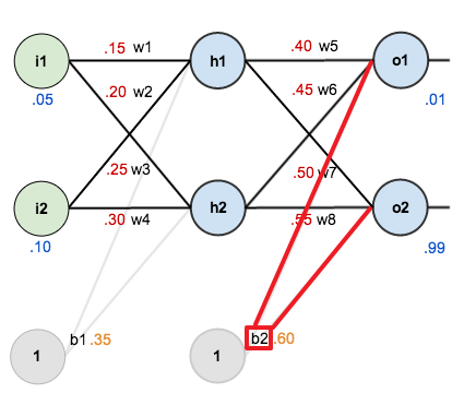
편향 $b_2$ 은 2개의 출력 노드 $o_1, o_2$ 에 영향을 주는 파라미터입니다.

따라서 $b_2$ 에 대한 전체 오차 $E_\text{total}$ 의 미분을 다음과 같이 나타낼 수 있습니다.

 

${ \partial E_\text{total} \over \partial b_2} = { \partial E_{o_1} \over \partial b_2} + { \partial E_{o_2} \over \partial b_2}$

 

각각 체인 룰을 적용합니다.

 

$\begin{aligned}
{ \partial E_{o_1} \over \partial b_2} & = { \partial E_{o_1} \over \partial out_{o_1} } { \partial out_{o_1} \over \partial net_{o_1} } { \partial net_{o_1} \over \partial b_2 } \\\\ 
& = 0.741365069 * 0.186815602 * 1 \\\\ 
& = 0.138498562
\end{aligned}$

 

$\begin{aligned}
{ \partial E_{o_2} \over \partial b_2} & = { \partial E_{o_2} \over \partial out_{o_2} } { \partial out_{o_2} \over \partial net_{o_2} } { \partial net_{o_2} \over \partial b_2 } \\\\ 
& = -0.217071535 * 0.175510053 * 1 \\\\ 
& = -0.038098237
\end{aligned}$

 

$\begin{aligned}
{ \partial E_\text{total} \over \partial b_2} & = { \partial E_{o_1} \over \partial b_2} + { \partial E_{o_2} \over \partial b_2} \\\\ 
& = 0.138498562 - 0.038098237 \\\\ 
& = 0.100400325
\end{aligned}$ 

 

경사 하강법을 적용해 $b_2$ 를 업데이트합니다.

 

$\begin{aligned}    
b_2^+ & = b_2 - \eta \, { \partial E_\text{total} \over \partial b_2 } \\\\     
& = 0.6 - 0.5 * 0.100400325 \\\\    
& = 0.549799838
\end{aligned}$

 

 

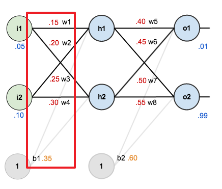
다음은 $w_1$~$w_4$, $b_1$ 에 대한 업데이트입니다.

$w_1$ 에 대한 기울기는 다음과 같이 나타낼 수 있습니다.

 

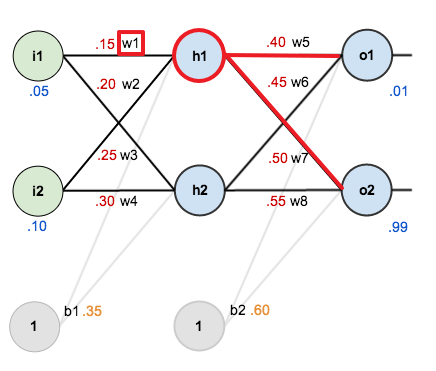
$ { \partial E_\text{total} \over \partial w_1 } = { \partial E_\text{total} \over \partial out_{h1} } { \partial out_{h_1} \over \partial net_{h_1} } { \partial net_{h_1} \over \partial w_1 } $

 

여기서 은닉층의 노드 $h_1$ 의 출력 $out_{h_1}$ 은 2개의 출력 노드 $o_1, o_2$ 에 영향을 줍니다.

따라서 다음과 같이 나누어 줄 수 있습니다.

 

$ { \partial E_\text{total} \over \partial w_1 } = \color{red}{ \partial E_\text{total} \over \partial out_{h1} } { \partial out_{h_1} \over \partial net_{h_1} } { \partial net_{h_1} \over \partial w_1 } $

 

${ \partial E_\text{total} \over \partial out_{h_1} } = { \partial E_{o_1} \over \partial out_{h_1} } + { \partial E_{o_2} \over \partial out_{h_1} }$

 

각각 체인 룰을 적용하면 다음과 같습니다. 

 

${ \partial E_{o_1} \over \partial out_{h1} } = { \partial E_{o_1} \over \partial out_{o_1} } { \partial out_{o_1} \over \partial net_{o_1} } { \partial net_{o_1} \over \partial out_{h_1} } $

 

${ \partial E_{o_2} \over \partial out_{h_1} } = { \partial E_{o_2} \over \partial out_{o_2} } { \partial out_{o_2} \over \partial net_{o_2} } { \partial net_{o_2} \over \partial out_{h_1} } $

 

 

위에서 계산한 내용은 다음과 같습니다.

 

${\partial E_{o_1} \over \partial out_{o_1}} = 0.741365069$

${\partial out_{o_1} \over \partial net_{o_1}} = 0.186815602$

${\partial E_{o_2} \over \partial out_{o_2}} = -0.217071535$

${\partial out_{o_2} \over \partial net_{o_2}} = 0.175510053$

 

 

다음 항을 계산합니다.

 

${ \partial E_{o_1} \over \partial out_{h_1} } = { \partial E_{o_1} \over \partial out_{o_1} } { \partial out_{o_1} \over \partial net_{o_1} } \color{red}{ \partial net_{o_1} \over \partial out_{h_1} } $

 

$ { \partial net_{o_1} \over \partial out_{h_1} } = {\partial \over \partial out_{h_1}} (w_5 * out_{h_1} + w_6 * out_{h_2} + b_2) = w_5 = 0.4 $

 

$ { \partial E_{o_1} \over \partial out_{h_1} } $ 을 계산합니다.

 

$\begin{aligned}
{ \partial E_{o_1} \over \partial out_{h_1} } & = { \partial E_{o_1} \over \partial out_{o_1} } { \partial out_{o_1} \over \partial net_{o_1} } { \partial net_{o_1} \over \partial out_{h_1} } \\\\
& = 0.741365069 * 0.186815602 * 0.4 \\\\
& = 0.055399425
\end{aligned}$

 

동일한 방식으로 ${ \partial E_{o_2} \over \partial out_{h_1} }$ 도 계산합니다.

 

$\begin{aligned}  
{ \partial E_{o_2} \over \partial out_{h_1} } & = { \partial E_{o_2} \over \partial out_{o_2} } { \partial out_{o_2} \over \partial net_{o_2} } { \partial net_{o_2} \over \partial out_{h_1} } \\\\  
& = -0.217071535 * 0.175510053 * 0.5 \\\\  
& = -0.019049118
\end{aligned}$

 

최종적으로 ${ \partial E_\text{total} \over \partial out_{h_1} }$ 은 다음과 같습니다.

 

$\begin{aligned}
{ \partial E_\text{total} \over \partial out_{h_1} } & = { \partial E_{o_1} \over \partial out_{h_1} } + { \partial E_{o_2} \over \partial out_{h_1} } \\\\
& = 0.055399425 - 0.019049118 \\\\
& = 0.036350307 
\end{aligned}$

 

다음 항을 계산합니다.

 

$ { \partial E_\text{total} \over \partial w_1 } = { \partial E_\text{total} \over \partial out_{h1} } \color{red}{ \partial out_{h_1} \over \partial net_{h_1} } { \partial net_{h_1} \over \partial w_1 } $

 

$ { \partial out_{h_1} \over \partial net_{h_1} } = out_{h_1} ( 1 - out_{h_1} ) = 0.593269992 ( 1 - 0.593269992 ) = 0.241300709 $

 

다음 항을 계산합니다.

 

$ { \partial E_\text{total} \over \partial w_1 } = { \partial E_\text{total} \over \partial out_{h1} } { \partial out_{h_1} \over \partial net_{h_1} } \color{red}{ \partial net_{h_1} \over \partial w_1 } $

 

$ { \partial net_{h_1} \over \partial w_1 } = { \partial \over \partial w_1 } ( w_1 * i_1 + w_2 * i_2 + b_1 ) = i_1 = 0.05 $

 

최종적으로 $ { \partial E_\text{total} \over \partial w_1 } $ 을 계산합니다.

 

$\begin{aligned} 
{ \partial E_\text{total} \over \partial w_1 } & = { \partial E_\text{total} \over \partial out_{h1} } { \partial out_{h_1} \over \partial net_{h_1} } { \partial net_{h_1} \over \partial w_1 } \\\\ 
& = 0.036350307 * 0.241300709 * 0.05 \\\\ 
& = 0.000438568
\end{aligned}$

 

경사 하강법을 적용하여 $w_1$ 을 업데이트합니다.

 

$\begin{aligned} 
w_1^+ & = w_1 - \eta \, { \partial E_\text{total} \over \partial w_1 } \\\\  
& = 0.15 - 0.5 * 0.000438568 \\\\ 
& = 0.149780716
\end{aligned}$

 

동일하게 가중치 $w_2, w_3, w_4$ 도 업데이트합니다.

 

$\begin{aligned}  
{ \partial E_\text{total} \over \partial w_2 } & = { \partial E_\text{total} \over \partial out_{h1} } { \partial out_{h_1} \over \partial net_{h_1} } { \partial net_{h_1} \over \partial w_2 } \\\\  
& = 0.036350307 * 0.241300709 * 0.1 \\\\  
& = 0.000877135
\end{aligned}$

 

$\begin{aligned}   
w_2^+ & = w_2 - \eta \, { \partial E_\text{total} \over \partial w_2 } \\\\   
& = 0.2 - 0.5 * 0.000877135 \\\\   
& = 0.199561432
\end{aligned}$

 

$\begin{aligned}    
{ \partial E_\text{total} \over \partial w_3 } & = { \partial E_\text{total} \over \partial out_{h2} } { \partial out_{h_2} \over \partial net_{h_2} } { \partial net_{h_2} \over \partial w_3 } \\\\    
& = 0.041370323 * 0.240613417 * 0.05 \\\\    
& = 0.000497713
\end{aligned}$

 

$\begin{aligned}     
w_3^+ & = w_3 - \eta \, { \partial E_\text{total} \over \partial w_3 } \\\\     
& = 0.25 - 0.5 * 0.000497713 \\\\     
& = 0.249751144
\end{aligned}$

 

$\begin{aligned}    
{ \partial E_\text{total} \over \partial w_4 } & = { \partial E_\text{total} \over \partial out_{h1} } { \partial out_{h_1} \over \partial net_{h_1} } { \partial net_{h_1} \over \partial w_4 } \\\\    
& = 0.041370323 * 0.240613417 * 0.1 \\\\    
& = 0.000995426
\end{aligned}$

 

$\begin{aligned}     
w_4^+ & = w_4 - \eta \, { \partial E_\text{total} \over \partial w_4 } \\\\     
& = 0.3 - 0.5 * 0.000995426 \\\\     
& = 0.299502287
\end{aligned}$

 

 

편향 $b_1$ 은 2개의 은닉층 노드 $h1, h2$ 에 영향을 주는 파라미터입니다.

따라서 $b_1$ 에 대한 기울기는 다음과 같이 구할 수 있습니다.

 

$\begin{aligned} 
{ \partial E_\text{total} \over \partial b_1 } & = { \partial E_\text{total} \over \partial out_{h_1} } { \partial out_{h_1} \over \partial net_{h_1} } { \partial net_{h_1} \over \partial b_1 } + { \partial E_\text{total} \over \partial out_{h_2} } { \partial out_{h_2} \over \partial net_{h_2} } { \partial net_{h_2} \over \partial b_1 } \\\\
& = 0.000438568 * 0.241300709 * 1 + 0.041370323 * 0.240613417 * 1 \\\\ 
& = 0.010060082 
\end{aligned}$

 

$\begin{aligned}       
b_1^+ & = b_1 - \eta \, { \partial E_\text{total} \over \partial b_1 } \\\\       
& = 0.35 - 0.5 * 0.010060082 \\\\       
& = 0.344969959
\end{aligned}$

 

 

여기까지 모든 파라미터에 대한 업데이트를 완료했습니다.

 

$\begin{aligned}
w_1^+ = 0.149780716 \\
w_2^+ = 0.199561432 \\
w_3^+ = 0.249751144 \\
w_4^+ = 0.299502287 \\
w_5^+ = 0.358916480 \\
w_6^+ = 0.408666186 \\
w_7^+ = 0.511301271 \\
w_8^+ = 0.561370121 \\
b_1^+ = 0.344969959 \\
b_2^+ = 0.549799838
\end{aligned}$

 

이제 업데이트된 파라미터를 이용해 다시 순전파를 통해 출력값을 계산합니다.

 

$\begin{aligned}
net_{h_1} & = w_1 * i_1 + w_2 * i_2 + b_1 \\\\
& = 0.149780716 * 0.05 + 0.199561432 * 0.1 + 0.344969959 \\\\
& = 0.372415138
\end{aligned}$

 

$ out_{h_1} = {1 \over {1 + e^{net_{h_1}}} } = {1 \over {1 + e^{ -0.372415138 }} } = 0.592042432$

 

$\begin{aligned}
net_{h_2} & = w_3 * i_1 + w_4 * i_2 + b_1 \\\\
& = 0.249751144 * 0.05 + 0.299502287 * 0.1 + 0.344969959 \\\\
& = 0.387407745 
\end{aligned}$

 

$ out_{h_2} = {1 \over {1 + e^{net_{h_2}}} } = {1 \over {1 + e^{ -0.3874077449 }} } = 0.595658511 $

 

$\begin{aligned}     
net_{o_1} & = w_5 * out_{h_1} + w_6 * out_{h_2} + b_2 \\\\     
& = 0.358916480 * 0.592042432+ 0.408666186 * 0.595658511 + 0.549799838 \\\\    
& = 1.005719116
\end{aligned} $

 

$ out_{o_1} = {1 \over {1 + e^{net_{o_1}}} } = {1 \over {1 + e^{ -1.005719116 }} } = 0.732181538 $

 

$ \begin{aligned}     
net_{o_2} & = w_7 * out_{h_1} + w_8 * out_{h_2} + b_2 \\\\     
& = 0.511301271 * 0.592042432 + 0.561370121 * 0.595658511 + 0.549799838 \\\\    
& = 1.186896776
\end{aligned} $

 

$ out_{o_2} = {1 \over {1 + e^{net_{o_2}}} } = {1 \over {1 + e^{ -1.186896776 }} } = 0.766185596 $

 

$ E_{o_1} = { 1 \over 2 } ( target_{o_1} - out_{o_1} )^2 = { 1 \over 2 } ( 0.01 - 0.732181538 )^2 = 0.260773087$

 

$ E_{o_2} = { 1 \over 2 } ( target_{o_2} - out_{o_2} )^2 = { 1 \over 2 } ( 0.99 - 0.766185596 )^2 = 0.025046444$

 

$ E_\text{total} = E_{o_1} + E_{o_2} = 0.260773087 + 0.025046444 = 0.285819531 $

 

 

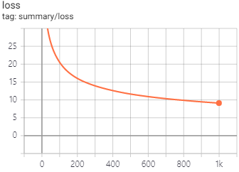
기존 오차와 비교해 감소되었습니다.

 

$ E_\text{old total} - E_\text{new total} = 0.298371109 - 0.285819531 = 0.012551578$